Assignment
The Office for Environmental Protection and Disaster Preparedness of the City of Stuttgart requires an integrated multi-hazard and climate-risk assessment for the urban area. Stuttgart's basin setting, the Neckar valley, the slopes at the edge of the city and the urban heat-island effect make the location particularly informative: six natural hazards have very different spatial effects here, and climate change will additionally alter the picture by 2050.
You are to carry out this analysis end to end—from data acquisition and the calculation of hazard indices to a publication-ready map composition and a written report. The assessment must answer four central questions:
- Topography and hazards: Which spatial patterns do the six natural hazards show across the urban area?
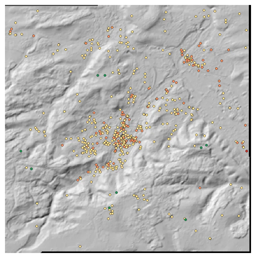
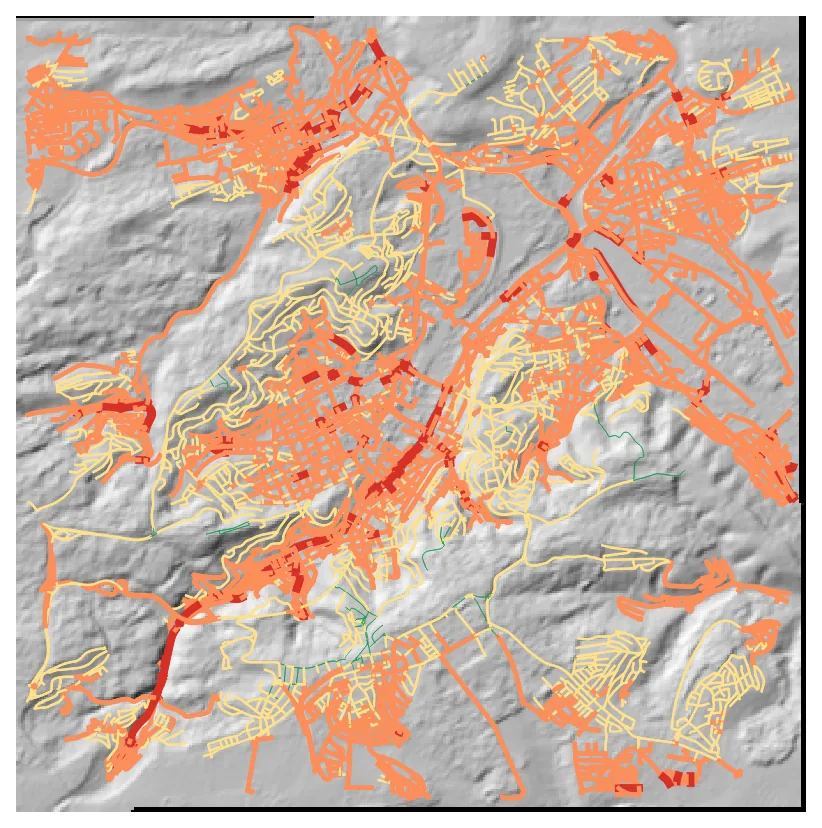
- Multi-geometry exposure: Which restaurants (points), buildings (polygons) and road sections (lines) are most exposed to flood risk?
- Statistics and composite assessment: How do the hazards correlate, how are their values distributed, and what does a weighted composite score look like?
- Climate projection: How does the risk picture shift under RCP 4.5 and RCP 8.5 by 2050?
Library recommendation and skill consultation
For geodata-based calculations, primarily use the geo-api library. Under
GeospatialRaster and GeospatialVector, it brings together precisely the data
sources (OSM, Microsoft Planetary Computer, DWD/CORDEX, Open-Meteo) and
algorithms (terrain derivatives, spectral indices, zonal statistics, routing)
required here. Read the geo-api skill before the first code action. Where
geo-api does not provide a direct algorithm—for example, specialised vector
operations or statistical aggregations—choose fallback packages yourself. The
skills geopandas-shapely, xarray-rioxarray, rasterio, grass-gis,
gdal-binaries, pyproj and qgis-styles are available and should be
consulted as needed.
For QGIS visualisation (layer tree, styling, screenshots, bookmarks, layout),
use the QGIS MCP bridge through the spatial-agent-bridge skill. You must
also consult the workflow skill bench (Coverage Tasks section); it describes
the RESULT.json schema and the screenshot self-review loop.
The choice of tools is explicitly yours—the prompt does not prescribe specific function or module names. In your initial plan, briefly explain which path you will take and why.
Procedure
Begin with a written plan of three to eight sentences in RESULT.json under
summary.plan: which phases you will complete and in what order, which skills
you have read and which data sources you will use. Only then begin the
implementation.
Create the directory structure early:
artifacts/
├── data/
│   ├── basemaps/
│   ├── osm/                  (restaurants, buildings, roads, districts)
│   ├── terrain/              (DEM and derivatives)
│   ├── hazards/              (6 hazard indices, composite and inundation zones)
│   ├── analysis/             (sampling results and aggregations)
│   └── climate/              (RCP-scaled results)
├── charts/                   (matplotlib PNG files)
└── screenshots/              (QGIS screenshots)
Save the QGIS project as artifacts/stuttgart_hazards.qgz. Set the project CRS
deliberately (EPSG:25832 is an appropriate choice for southern Germany).
Phase 1—Define the study area and acquire base data
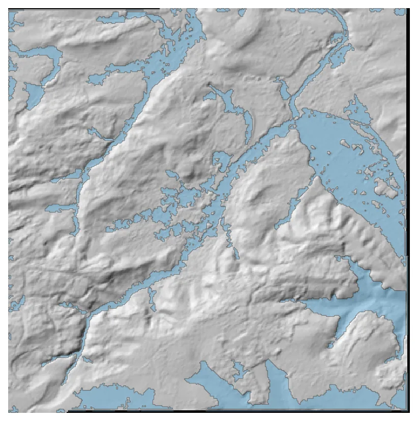
Define the study area: the City of Stuttgart together with the surrounding ridges (Bopser, Killesberg, Frauenkopf), covering a bounding box of approximately 10 × 10 km. Obtain for this area:
- a digital elevation model at approximately 30 m resolution (Copernicus GLO-30 via Microsoft Planetary Computer is the standard choice);
- an OSM basemap layer;
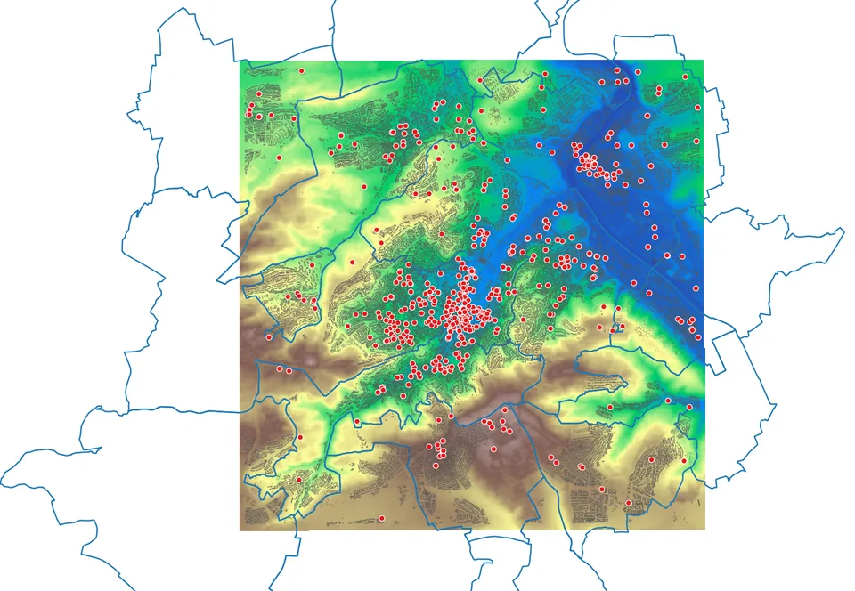
- OSM vector data: all restaurants (POIs), all building polygons, the drivable road network and the city-district boundaries.
DEM acquisition note: download only the area-of-interest subset, not complete tile stacks.
Organise the downloaded layers in QGIS in a meaningful layer tree, using groups
such as “Terrain/Source data”, “Urban/Buildings”, “POI”,
“Administration/Districts” and “Basemaps”. Style examples from the
qgis-styles skill are welcome.
Create an overview screenshot at the end of the phase.
Phase 2—Terrain derivatives
The principal terrain derivatives must be produced from the DEM. At minimum, these are:
- slope in degrees;
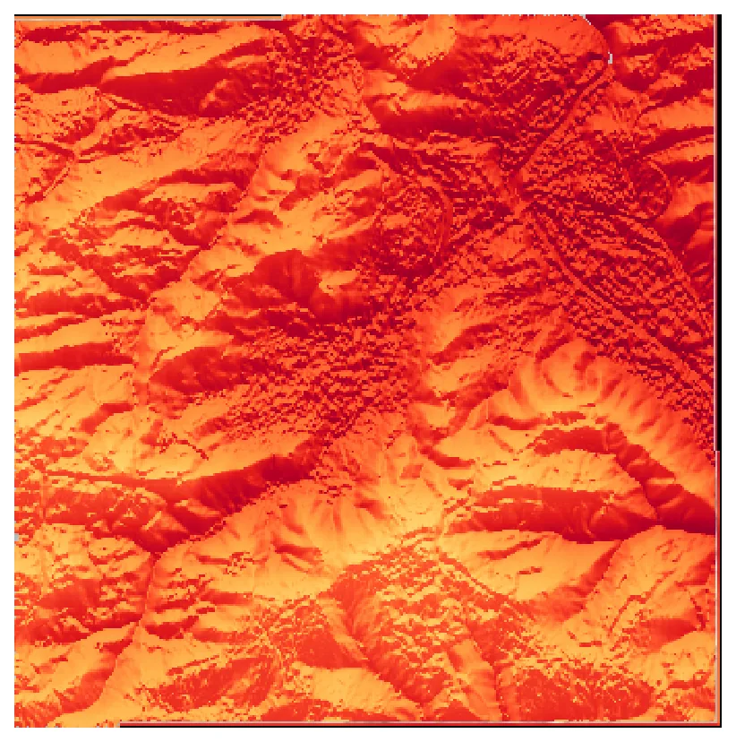
- aspect from 0–360°;
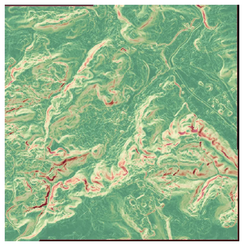
- topographic position, for example TPI at an approximately 330 m window radius;
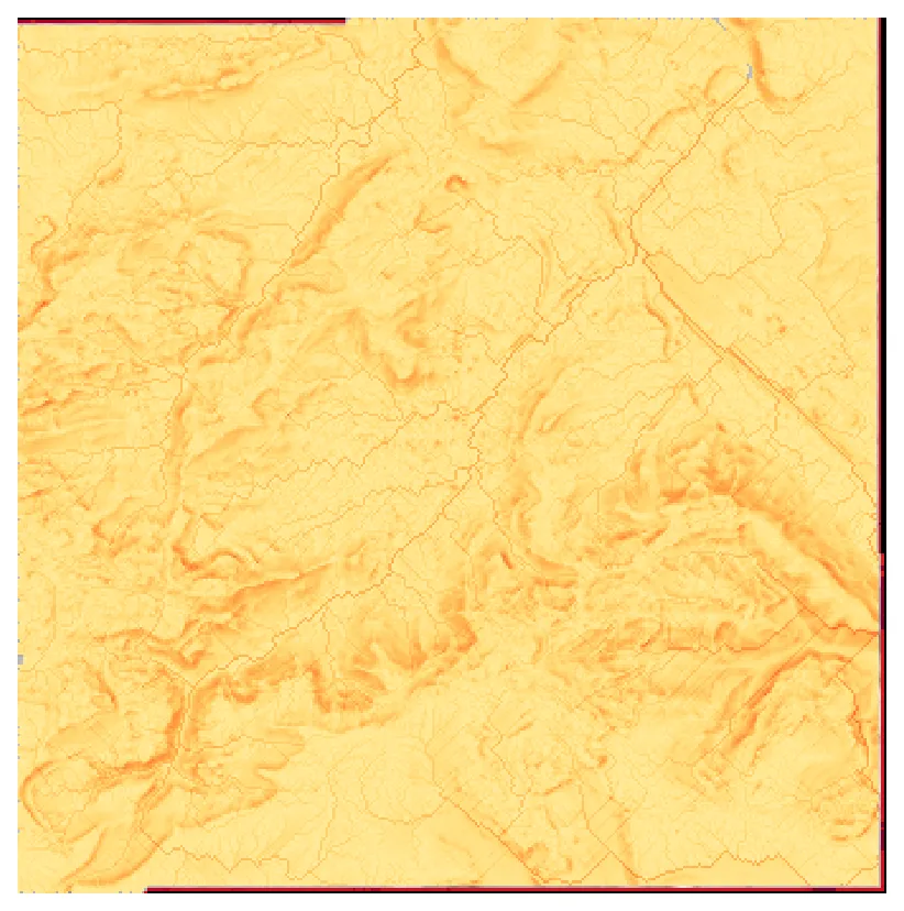
- topographic wetness index, for example TWI;
- ruggedness, for example TRI;
- profile curvature;
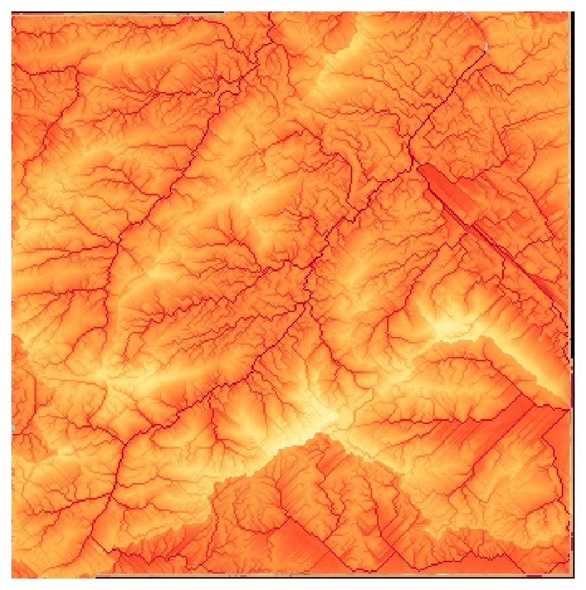
- height above nearest drainage, or HAND;
- flow accumulation;
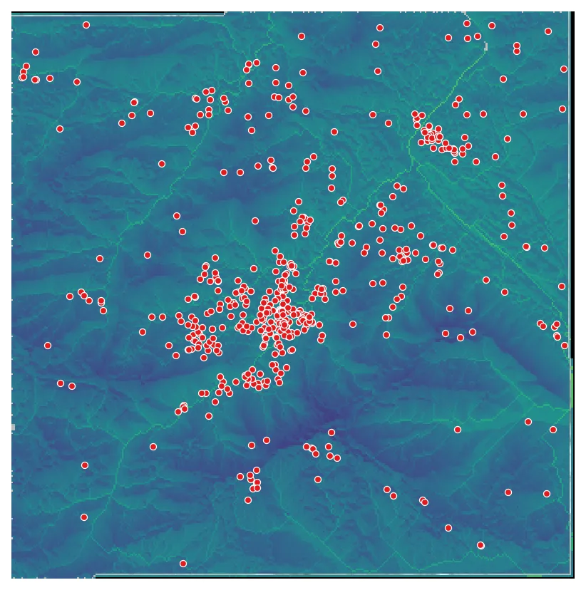
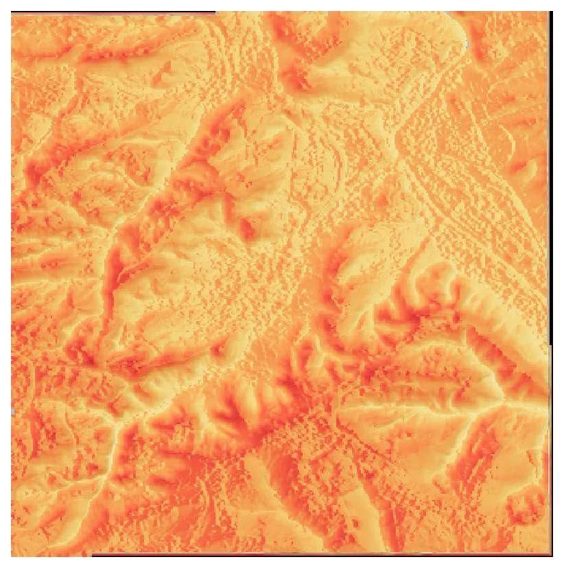
- hillshade for visualisation.
The library or tool used is open: geo-api provides a terrain accessor for
many of these calculations, GRASS GIS offers specialised modules (see the
grass-gis skill), and the GDAL CLI provides several fundamentals (see the
gdal-binaries skill). HAND is usually the most demanding step, comprising flow
accumulation, stream extraction and vertical distance.
Performance note: Watershed algorithms, particularly HAND and flow
accumulation, can consume several tens of gigabytes of RAM for a 10 × 10 km,
30 m DEM when implemented naively in Python. If you notice that a process uses
more than 20 GB RSS, stop it and change approach. GRASS GIS r.watershed is
considerably more memory-efficient on large DEMs than Python alternatives
because it uses time-tested C code. Alternatively, downsample the DEM to about
60 m before computing HAND; doubling the cell size quarters the pixel count.
Document the chosen approach under summary.hazard_formulas.
Style the derivatives so the information is clear: hillshade as a greyscale background; slope in warm colours; TPI with a diverging valley-to-ridge scale; TWI sequentially from dry to wet; and HAND sequentially from near drainage to high above it.
Create a screenshot of the derivative overview; hillshade with a semi-transparent slope layer is a useful default.
Phase 3—Six hazard indices and a composite
Calculate six normalised hazard indices from the terrain derivatives, each scaled to [0,1], where 1 indicates the greatest hazard, and a weighted composite. The following indices and physical rationales are expected:
| Index | What it models | Recommended components |
|---|---|---|
| Wind exposure | Ridges and west-facing slopes are exposed to wind | TPI, west-facing measure, relative elevation, slope |
| Frost risk | Cold air pools in valleys and wet depressions | Valley position (inverse TPI), TWI, low relative elevation |
| Flood risk | Low-lying areas near drainage with large catchments | Inverse HAND, TWI, flow accumulation |
| Heat stress | Low elevation, south-facing slope and urban factor | Inverse elevation, south-facing measure, urban factor (constant) |
| Landslide | Steep, wet and concave terrain | Slope, TWI, concavity |
| Erosion (LS factor) | RUSLE LS factor from flow and slope | Flow accumulation, slope function |
The exact formulas and weights are at your discretion. Follow standard
literature—for example RUSLE for erosion, TPI for wind and HAND for flooding—and
document the selected formulas in RESULT.json under
summary.hazard_formulas.
Composite: a weighted sum of the six indices. Choose and justify the weights; flood and heat would typically receive greater weight in an urban heat and flooding context.
Screenshots: create a separate map over hillshade for each signature hazard (wind, flood, heat and landslide), plus a composite overview map.
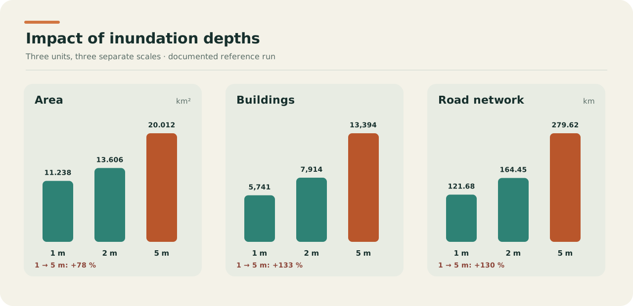
Also create HAND-based inundation zones for three scenarios: water levels of 1 m, 2 m and 5 m above the nearest drainage. Export the zones as polygons, for example to a GeoPackage. For each scenario, calculate and report inundated area in km², number of affected buildings and total length of affected roads in km.
Phase 4—Multi-geometry exposure
Three geometry types must be sampled with hazard values. This is deliberate, because each requires a different raster-to-vector extraction method:
- Restaurants (points): extract all six hazard values plus elevation and slope for each point. Calculate a composite score for each restaurant using weights of your choice and document those weights. Assign four risk classes: Low, Medium, High and Very High.
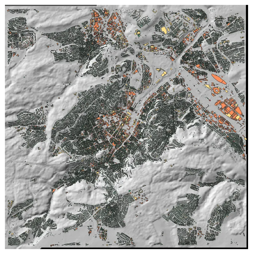
- Buildings (polygons): aggregate the flood index for each polygon using zonal statistics or centroid sampling, choosing the method that is appropriate. Assign four risk classes.
- Roads (lines): similarly aggregate the flood index for each segment. Assign four risk classes and use line width proportional to the score in the visualisation.
Export all three result sets as separate GeoPackages under
artifacts/data/analysis/. Also export the restaurant results as GeoJSON and
CSV.
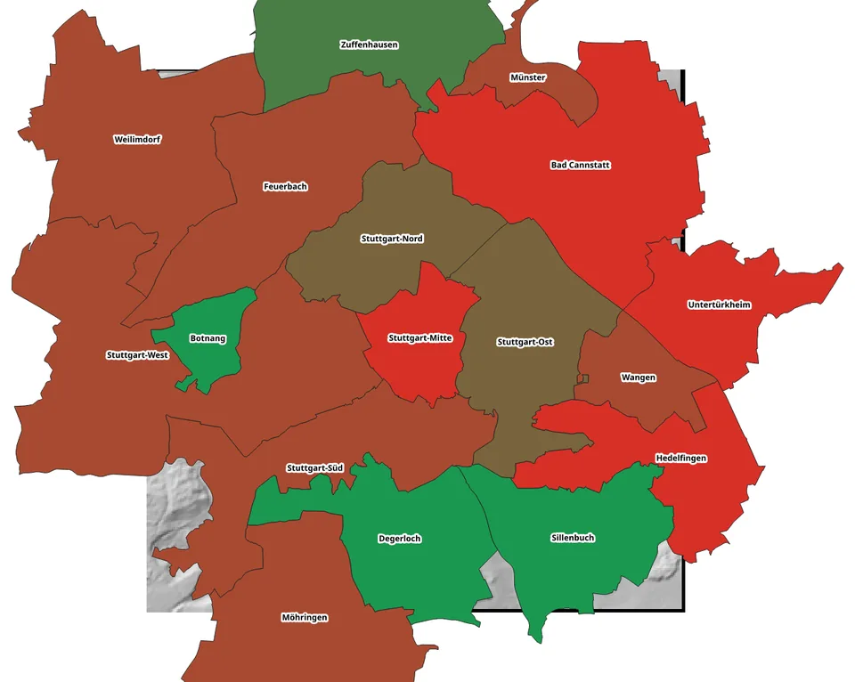
District-level aggregation: spatially join restaurants to city districts, calculate the mean, count and percentage at high risk per district, and visualise the result as choropleth polygons in QGIS.
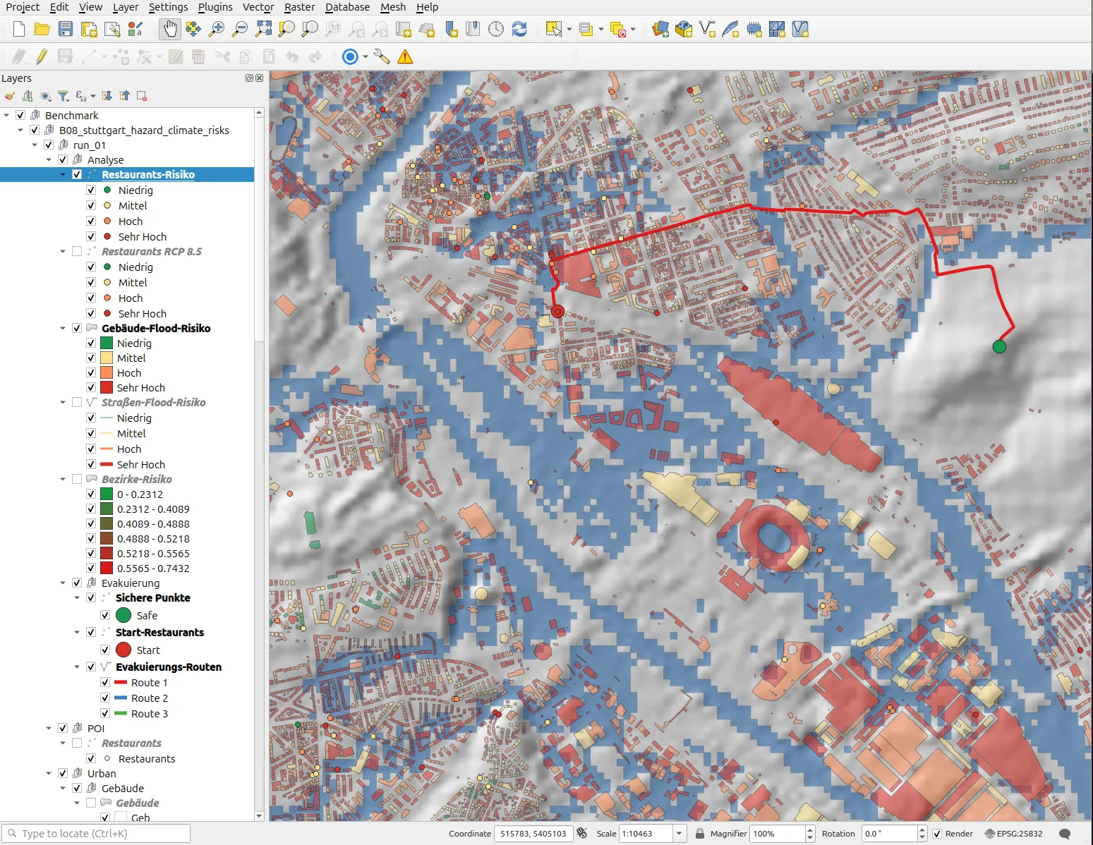
Screenshots: one dedicated screenshot per geometry type—restaurants, buildings and roads styled by risk class—plus a district choropleth and the three inundation zones.
Phase 5—Statistics and charts
Generate at least seven charts as PNG files under artifacts/charts/.
The minimum inventory is:
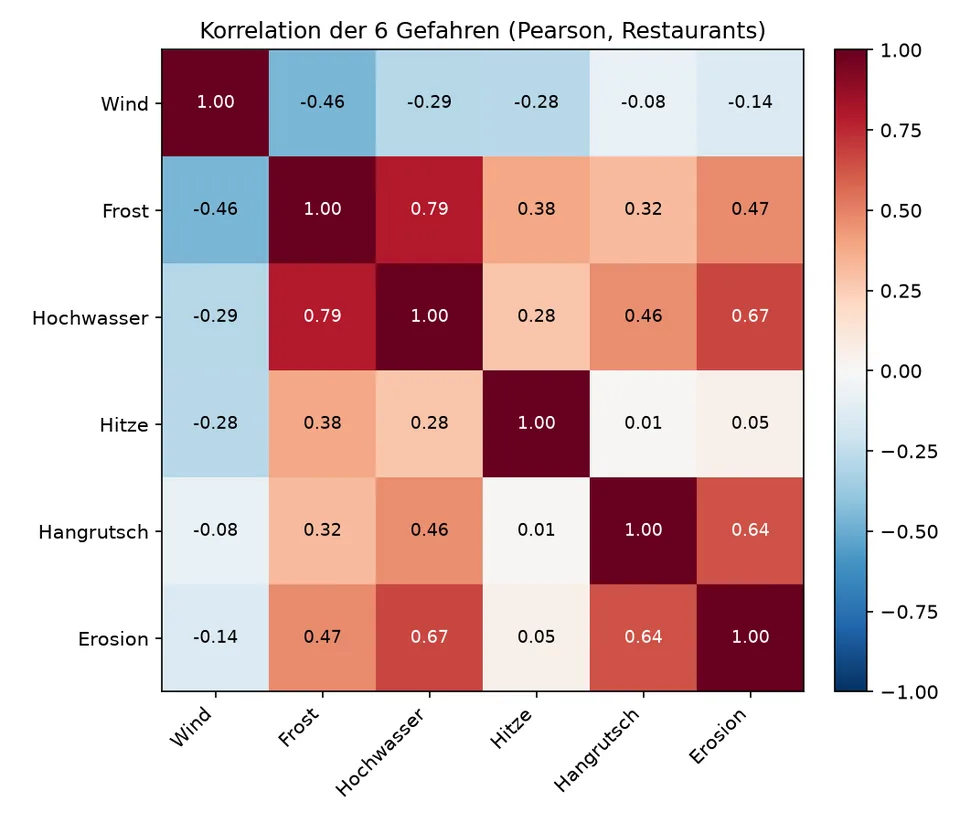
- correlation heatmap for the six hazards across all restaurants (6 × 6, Pearson, diverging colour scale with annotated values);
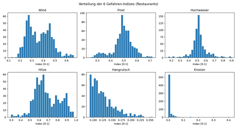
- histogram panel for the six hazards, showing the shape of each distribution;
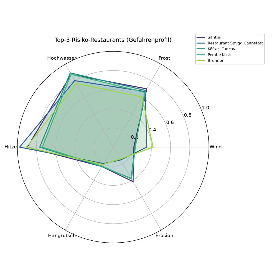
- radar charts for the five restaurants with the highest risk;
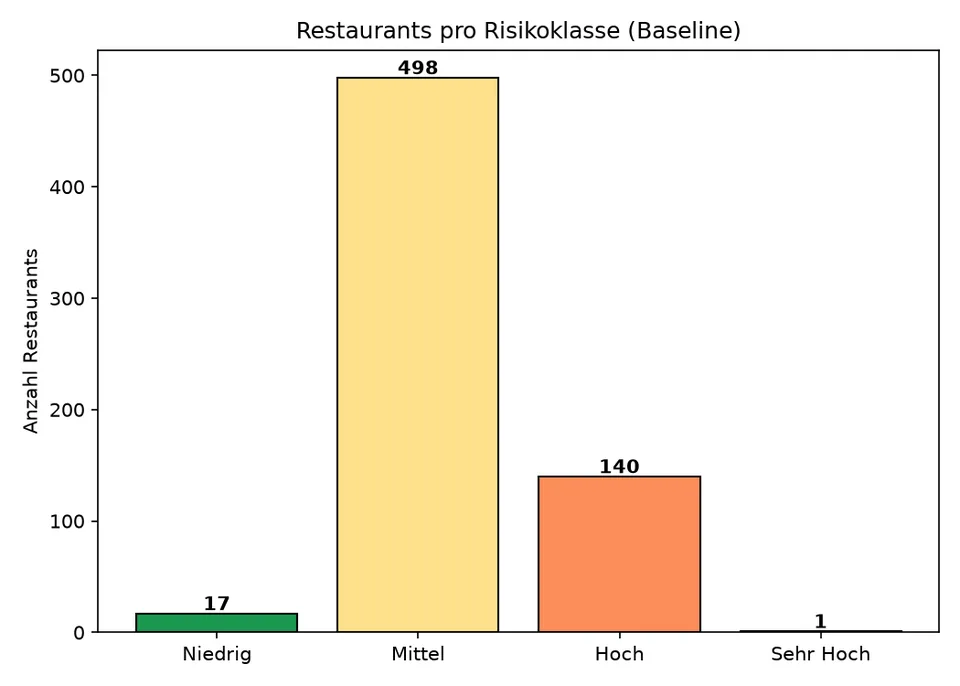
- bar chart of restaurant count by risk class;
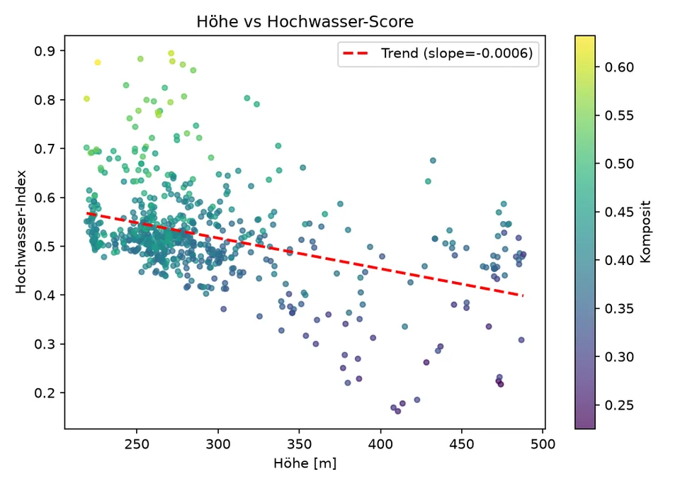
- scatter plot of elevation versus flood score, with trend line;
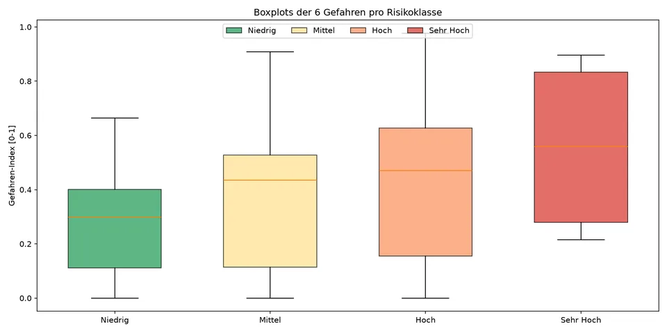
- box plots of all six hazards by risk class;
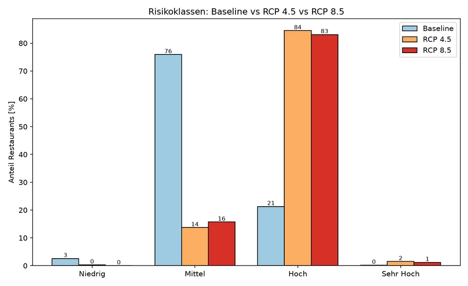
- climate-comparison bar chart for baseline, RCP 4.5 and RCP 8.5.
Chart 7 will be calculated in Phase 7, but its skeleton may already be prepared here.
Phase 6—High-risk inspection and evacuation routing
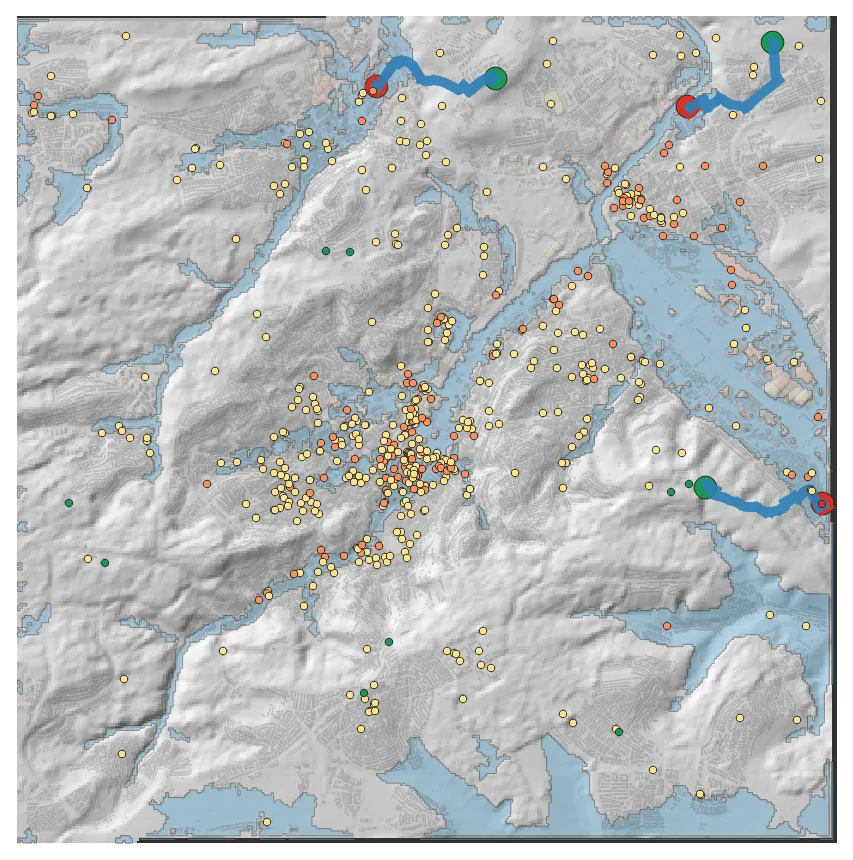
Select restaurants with a composite score above 0.50. Zoom to the spatial cluster with the greatest concentration and to the single restaurant with the highest score, producing a separate screenshot of each.
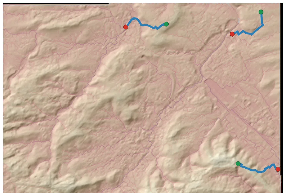
Select the three restaurants with the highest composite score and calculate a
pedestrian route from each to a safe point, for example a point with HAND above
10 m on a ridge. Routing may use OSM: geo-api provides a routing component, or
OSMnx may be used for graph-based routing; consult the corresponding skills.
Identify route segments that cross flood-prone areas with a flood index above 0.5; these are vulnerable segments. Report route length, estimated walking time and vulnerable share.
Create a screenshot of the three routes with the vulnerable segments highlighted.
Phase 7—Climate projection (RCP 4.5 and RCP 8.5, 2050 horizon)
Apply climate-scaling factors to each restaurant’s baseline hazard values. The following are indicative values for the CORDEX ensemble to 2050 in southern Germany:
| Hazard | RCP 4.5 factor | RCP 8.5 factor | Direction |
|---|---|---|---|
| Wind | ~1.00 | ~1.00 | static |
| Frost | ~0.77 | ~0.55 | decreasing |
| Flood | ~1.03 | ~1.07 | slightly increasing |
| Heat | ~1.80 | ~2.59 | strongly increasing |
| Landslide | ~1.00 | ~1.00 | static |
| Erosion | ~1.03 | ~1.07 | slightly increasing |
You may use these factors directly (source: EURO-CORDEX EUR-11,
MPI-M-MPI-ESM-LR, 2050) or retrieve more detailed values through
geo_api.ClimateDataApi if that better suits your workflow. Document the
factors used in RESULT.json.
For every restaurant, scale each hazard and cap it at 1.0, recalculate the
composite and assign the new risk class. Save the results as CSV files under
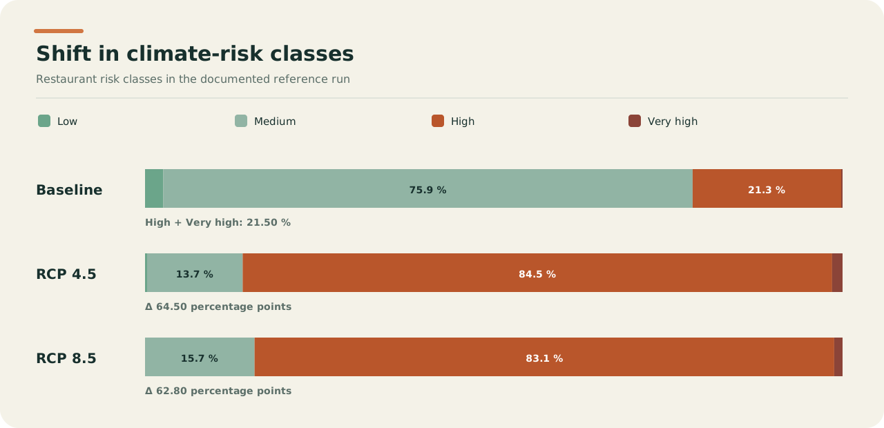
artifacts/data/climate/. Report the class shift as a percentage in each class
for each scenario.
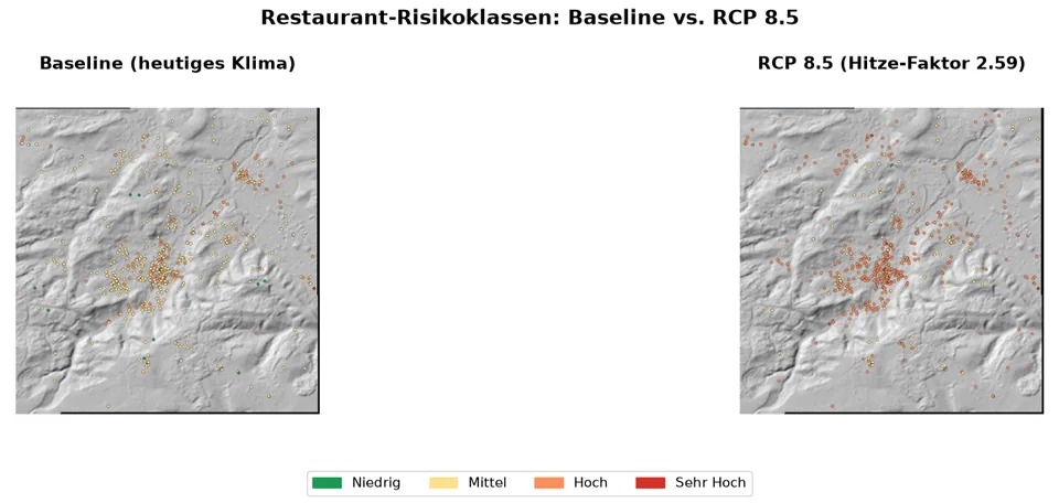
Generate Chart 7 from the actual data. Screenshot: display restaurants at baseline and under RCP 8.5 side by side in QGIS.
Phase 8—Finalisation
Clean up the layer tree for publication, with a clear hierarchy: analysis results at the top, hazards in the middle, and source data and basemap at the bottom.
Create a final composite screenshot with hillshade, a semi-transparent 2 m inundation zone, buildings by flood risk, restaurants by composite risk class and visible evacuation routes.
Write a report at artifacts/RESULTS.md in German or English with the usual
sections: executive summary, study area, method, results for each phase,
climate projections and recommendations. Embed the charts using Markdown.
Self-review loop for every screenshot
Follow skill bench, PROTOCOL §10 (Coverage Tasks): inspect every screenshot
before proceeding. If you are Claude Code, open the PNG with the Read tool and
inspect it visually. If you are Codex, use Bash with Python/PIL to check the
pixel distribution; a standard deviation below 5 suggests an empty or uniform
image. If a screenshot does not meet the expectation—because it is empty,
incorrectly centred, shows the wrong visible layers or is identical to the
previous phase—correct it and capture it again. Use no more than two retries per
phase. Document retries in RESULT.json under summary.review_notes[].
Screenshot rules (binding)
- After every
load_project, first perform amap_navigationaction such aszoom_to_layerorset_extentbefore taking the first screenshot. The canvas extent is undefined after loading a project in this environment and would otherwise produce an empty image. - Always call
get_map_screenshotwith explicit dimensions:width=1600, height=1000(default 96 dpi). Window geometry is unreliable in this environment; never rely on the canvas size. - Never use
include_overlays=true: the widget-grab path produces empty images in this environment. Map tips are not required for this task. - Check the
content_hashreturned after every screenshot. If it is identical to the preceding screenshot, the map has not changed and visibility or extent is incorrect; then apply the self-review loop.
What RESULT.json must contain
The RESULT.json must comply with the schema in the bench skill
(PROTOCOL.md). At the top level it requires task_id, run_index, mode,
summary, hard_checks and anti_checks. For every anti.never: rule in
this task, an anti_checks[] entry with id, violation and evidence must
exist. A missing entry is scored as a violation.
Under summary:
plan: the initial plan string described above;phases_completed: array["1", "2", ..., "8"];data_sources_used: list of data-source endpoints with versions, for example{"copernicus_glo30": "dem 1.0", "osm_overpass": "<date>"};hazard_formulas: dictionary with the selected formulas and weights for each hazard;climate_factors_used: dictionary with scaling factors by hazard for RCP 4.5 and RCP 8.5;composite_weights: dictionary with composite-score weights by geometry type;screenshots_written: list of relative paths;charts_written: list of relative paths;inundation_stats: dictionary for each scenario, for example{"1m": {"area_km2": ..., "buildings_affected": ..., "streets_km_affected": ...}, "2m": {...}, "5m": {...}};risk_class_distribution: dictionary{"baseline": {"Low": <pct>, "Medium": <pct>, "High": <pct>, "Very High": <pct>}, "rcp45": {...}, "rcp85": {...}};top_10_risk_restaurants: list with name or ID, district, composite score and dominant hazard;evacuation_routes: list with start restaurant, target coordinate, route length in metres, walking time in minutes and vulnerable kilometres;failures: array of{phase, action, error}for each unsuccessful step;review_notes: documentation of the self-review loop;abort_reason: string or null.
Final cleanup
All temporary QGIS layers, groups, bookmarks and layouts belong under the tree
node Benchmark/B08_stuttgart_hazard_climate_risks/run_<N> so that the next run
starts from a clean state. File outputs under artifacts/ remain in place; they
are the result of the task.