Fundamentals
How SpatialAgents work.
Thirteen sections lead from the idea of a coding agent to the measured result. They are written for anyone who works with QGIS and wants to know what happens between the task and the map. Every section has a graphic, a text and its spoken version; listening to all of them takes about a quarter of an hour.
Overview
Thirteen sections in four groups.
The order leads from the terms through the domain context to the system and ends at the evidence.
- 01What is a coding agent?Basics
- 02Tool useBasics
- 03Command line and open-source GISBasics
- 04MCP serversBasics
- 05Instruction filesDomain context
- 06SkillsDomain context
- 07Agentic planningDomain context
- 08One task, start to finishSystem
- 09Geospatial API and token efficiencySystem
- 10Plugin and bridgeSystem
- 11Control and computeSystem
- 12Local or cloudOperation and evidence
- 13Evidence through measurement seriesOperation and evidence
Total listening time: 19 min 58 s.
Concept 01 · Basics
What is a coding agent?
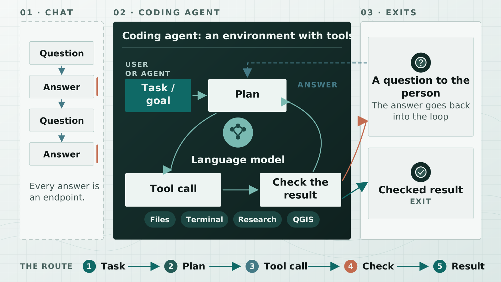
A chat runs as a chain of question and answer, and every answer is an endpoint.
A coding agent is not a language model but a working environment with a language model inside. The environment provides the tools: reading and writing files, running commands and looking things up. And it provides the loop, which leads from the task through the plan to a tool call, checks the result and returns to the plan.
Inside that loop the model plans, calls a tool and reads the result. If the first route fails, it tries another and plans again.
The loop ends at a checked, usable result or at a question to the person. A check alone does not end it, and after an answer it carries on.
A single run can take several hundred tool calls and last more than two hours without anyone intervening; permission is granted once at the start, not at every step.
Nobody has to build such an environment; they come ready-made.
Evidence
Concept 01 · part 2
Three coding agents: Claude Code, Codex CLI, OpenCode
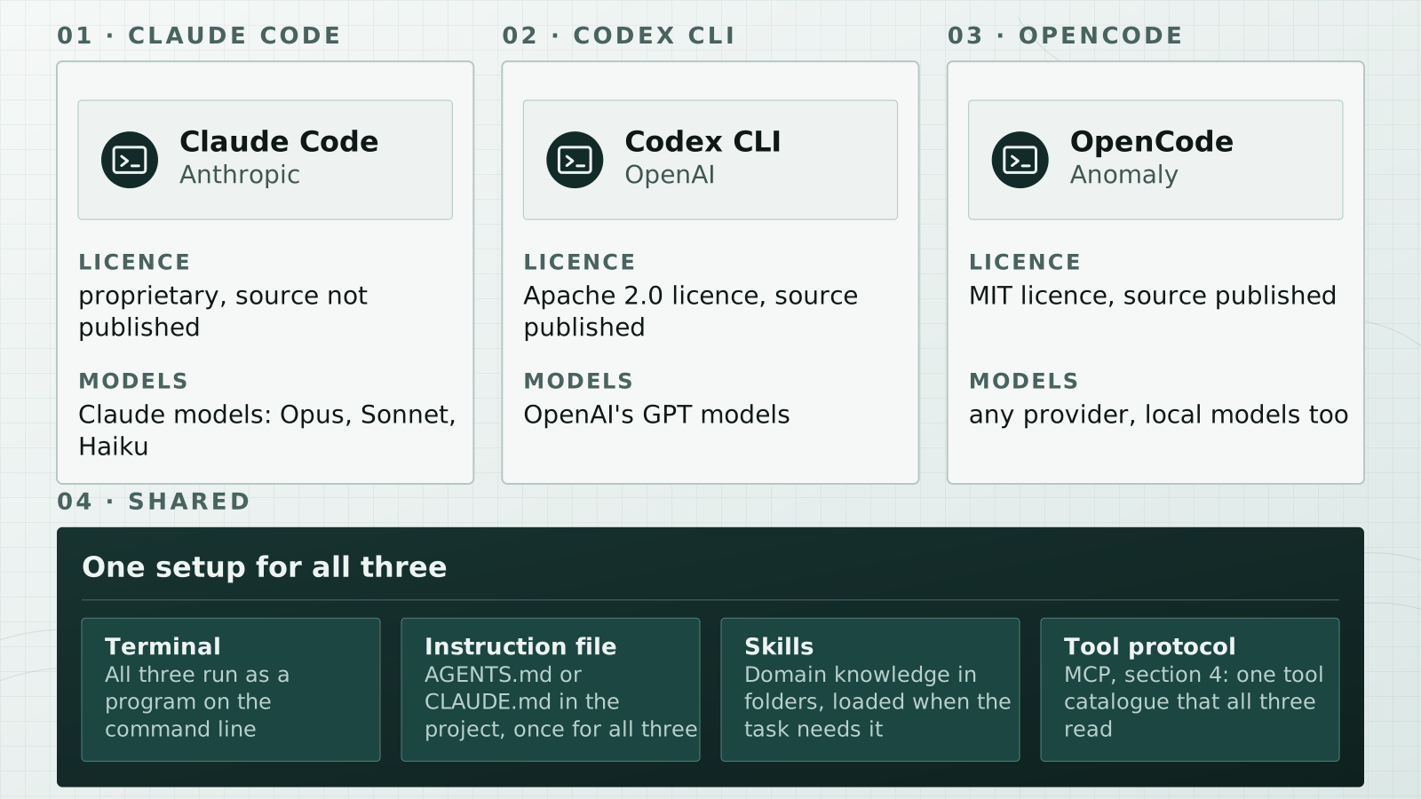
SpatialAgents work with three ready-made coding agents.
Claude Code comes from Anthropic; its source is not published, and it works with the Claude models. Codex comes from OpenAI, its source is free under the Apache 2.0 licence, and it works with the GPT models. OpenCode comes from Anomaly, likewise open under the MIT licence; it is tied to no provider and also works with a model that runs on your own machine.
All three run in the terminal, read the same instruction file in the project, load skills and connect tools by the same protocol. So one setup serves all three.
The measurement series ran seven models, which go by short names from here on. Opus, Sonnet and Haiku ran in Claude Code, Sol, Terra and Luna in Codex, and Qwen as the local model in OpenCode.
What a tool call actually looks like is still open.
Evidence
Concept 02 · Basics
Tool use
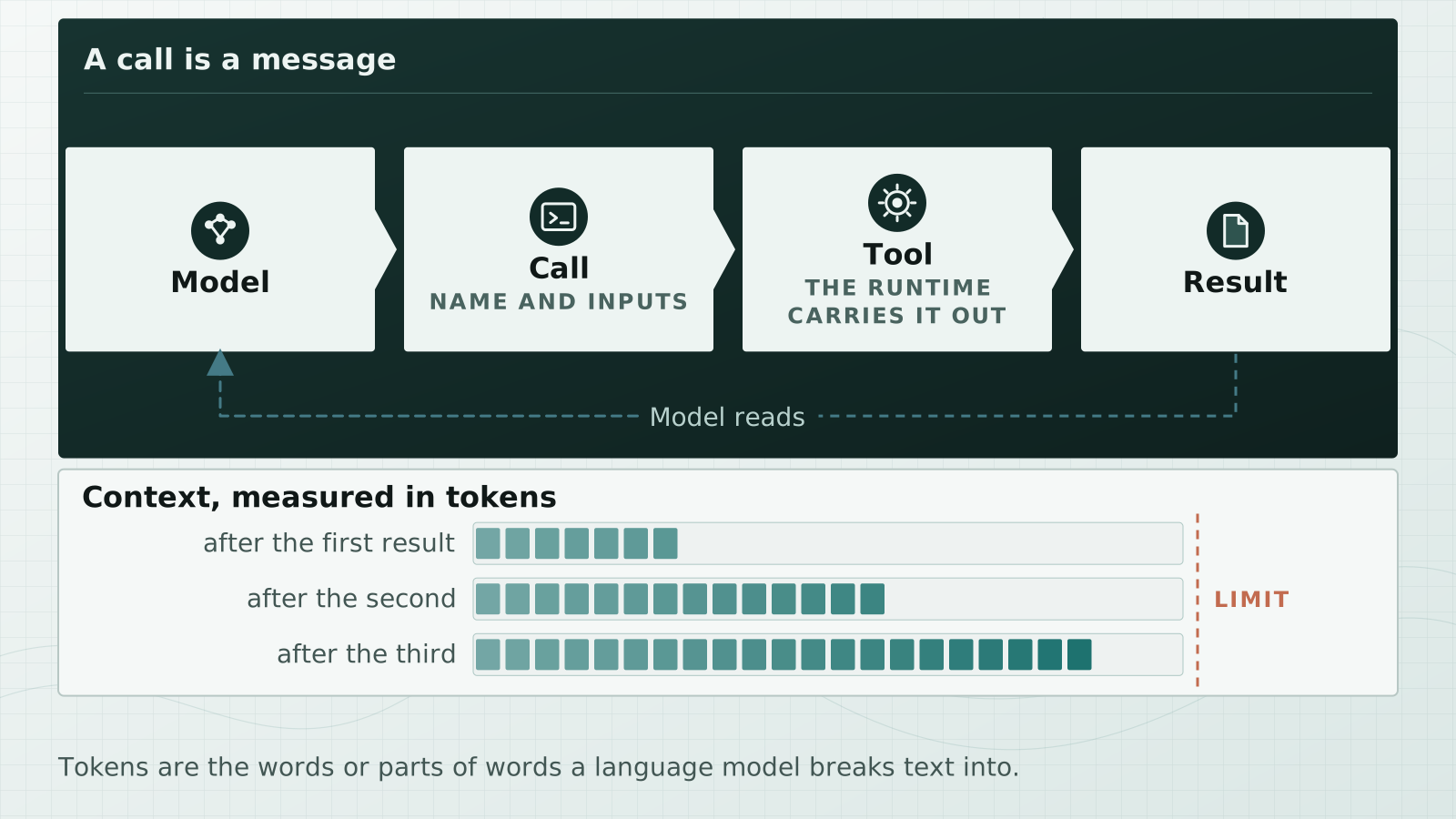
A language model cannot carry anything out; it can only write. A tool call is therefore a message with a fixed structure that names the tool and its inputs, and the environment runs the tool and writes the result back.
That result lands in the context, the text the model has in front of it at every step. The context is limited.
It is measured in tokens. A token is a word or a part of a word, and a language model reads and writes in such units.
Every result takes up part of the context, so what counts is how much a tool gives back.
How much that adds up to depends on the model. On the same task the mean use of a single run ranges from three million to almost a hundred million tokens, and the higher figure does not mean the better map.
For geodata, such tools do not have to be built first; they have existed for decades.
Evidence
Concept 03 · Basics
Command line and open-source GIS
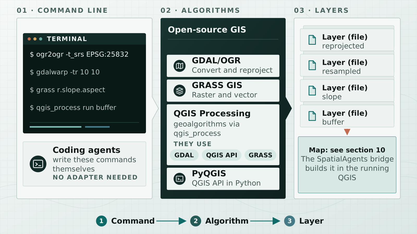
Open-source GIS tools have one property that is decisive for agents: you operate them with text.
On the command line, GDAL and OGR read, write, reproject and clip geodata with a single command, and GRASS GIS brings its modules in the same form. QGIS Processing runs its geoalgorithms through the command qgis_process. Those algorithms in turn drive GDAL, the programming interface of QGIS or GRASS modules. Anyone who prefers Python writes the same work with PyQGIS as a script.
A coding agent writes exactly such commands, and no translator is needed in between, because the tool is already there.
What such a command produces is a file, called a layer in the trade, a single plane of data. A layer holds geometries or raster cells and their values, but it is not a picture yet. The map is made in QGIS, and that is a step of its own.
So one thing is still missing: the way to QGIS itself.
Evidence
Concept 04 · Basics
MCP servers
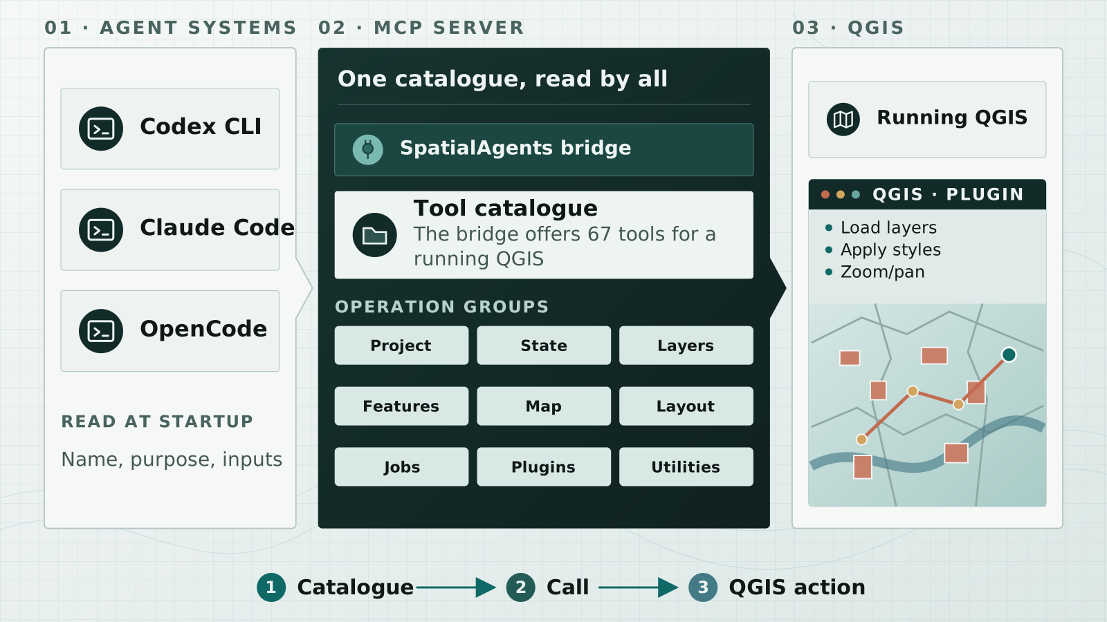
For an agent to operate an application, it needs a list of its tools. The Model Context Protocol, MCP for short, lays down how an application supplies that list.
Every entry names three things: the name of the tool, what it is good for and which inputs it expects.
An agent reads this list as soon as it starts. From then on it sits in the context, and it knows what the application can do.
For QGIS there is such a server, the SpatialAgents bridge. It offers 67 tools arranged in nine groups. They reach from opening a project and reading its state, through loading layers and querying their features, to the map, the print layout and longer-running jobs. The bridge runs as a process on the same machine as QGIS.
That settles which tools are available. How work is done in a project is written in a file of its own.
Evidence
Concept 05 · Domain context
Instruction files
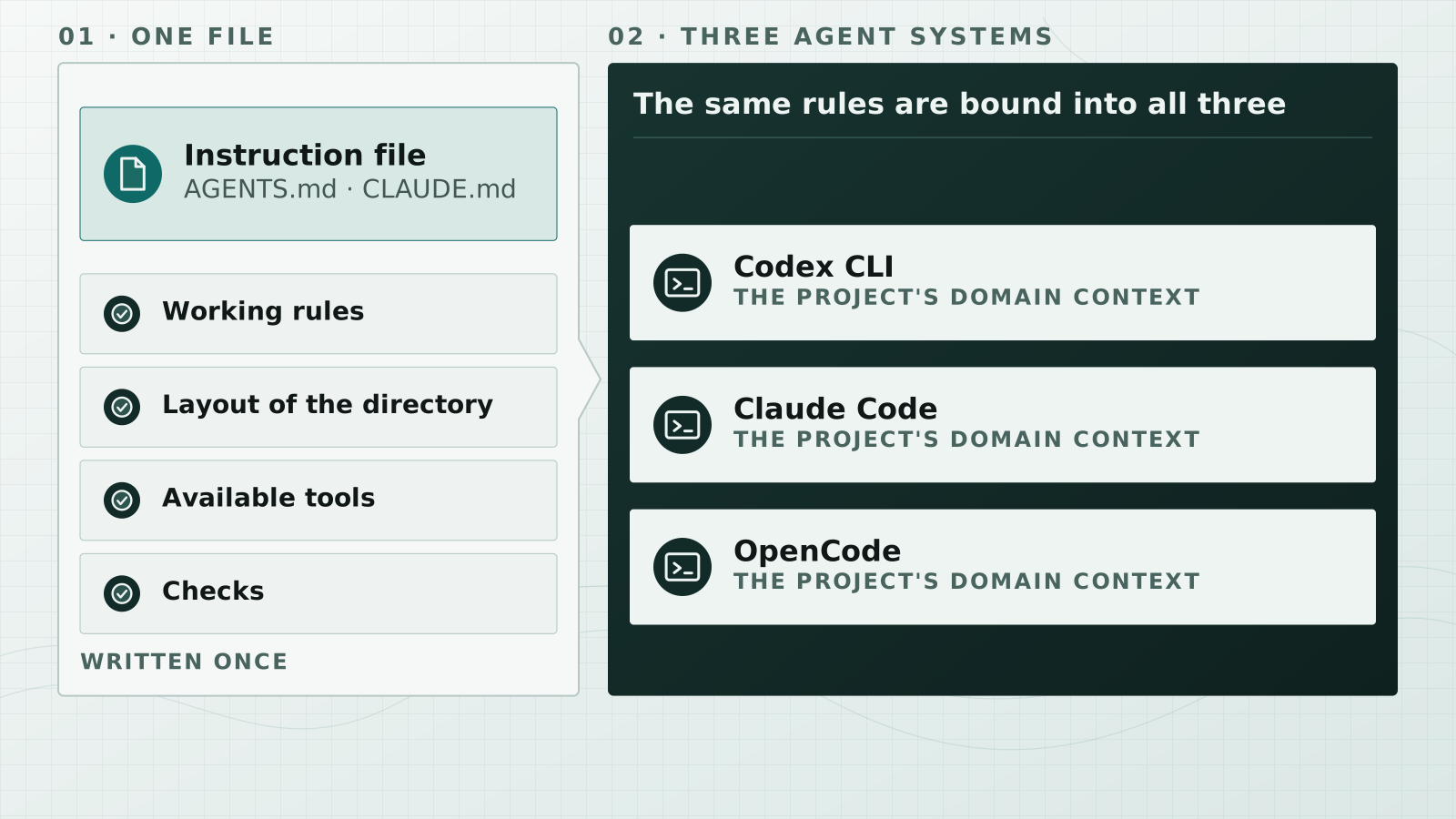
Before an agent works, it reads a file of instructions that lies in the project; each of the three coding agents knows such a file under its own name. It says how work is done in the project.
Four things are usually in it: the rules of the work, the layout of the directory, the available tools and the checks a result has to pass.
In SpatialAgents this domain context exists only once. Codex, Claude Code and OpenCode read the same text and work to the same rules, and changing the way of working means changing one file instead of three configurations.
That holds for the whole project. Domain knowledge for single tasks sits elsewhere and is loaded only when it is needed.
Evidence
Concept 06 · Domain context
Skills
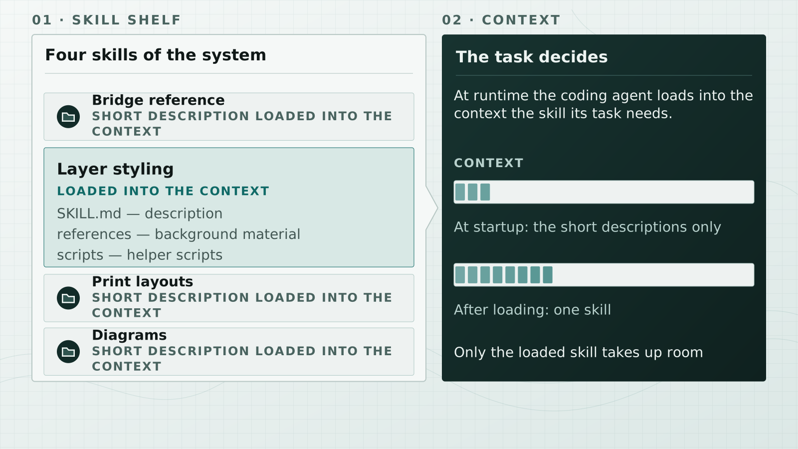
A skill is domain knowledge in a folder: a description, plus references and scripts. An agent system reads only the descriptions to begin with, and only when a task fits a skill does it load it into the context.
The gain lies in the context, because what is not loaded takes up no room.
Four skills belong to the system. The first describes the tools of the bridge, the second the styling of layers, the third the print layouts and the fourth the diagrams in the map.
The user says in ordinary language what they need, and the domain knowledge for it sits in the skill; nobody has to know QML or the internals of a layout.
That describes what an agent system knows. How it turns this into a plan for a large task is what agentic planning shows.
Evidence
Concept 07 · Domain context
Agentic planning
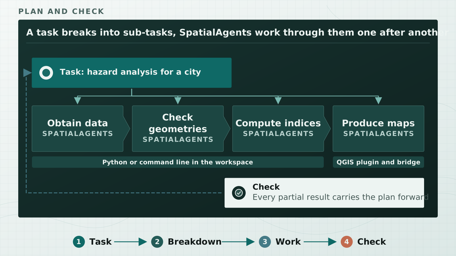
A hazard analysis for a city is not a single-step task. SpatialAgents break it down into four sub-tasks, namely obtain data, check geometries, compute indices and produce the map, and they lay this breakdown down as a plan. They work through the four sub-tasks one after another: three of them with Python or on the command line in the workspace, the map through the QGIS plugin and the bridge. The plan stays at the centre of the work and is carried forward after every partial result. A check that does not add up leads back to the task and produces a further step. The plan comes before the work begins.
Evidence
- Benchmark 08: task in eight phases, plan before the work, at most two retries per phase
- Benchmark 08: criterion “Initial plan present and traceable”, 5 points
- Claude Code: plan mode in the common workflows
- Codex CLI: documentation, planning before the change
- OpenCode: agent documentation with the plan agent
Concept 07 · part 2
The plan comes before the work
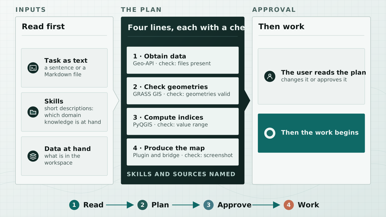
Before a coding agent touches a file, it reads. It reads the task, the short descriptions of the skills and the data in the workspace.
Then it writes the plan. The plan names the sub-tasks in their order. For every sub-task it names the tool and the check the sub-task ends with. And it names the skills and data sources it uses for that.
All three coding agents know this step. Claude Code has plan mode for it: the coding agent reads and proposes a plan but changes nothing until the user approves. OpenCode ships a plan agent of its own that only reads. Codex names planning as the first step before any change.
The user reads the plan, changes it or approves it. Only then does the work begin.
Every line of the plan ends with a check.
Evidence
Concept 07 · part 3
Every sub-task ends with a check
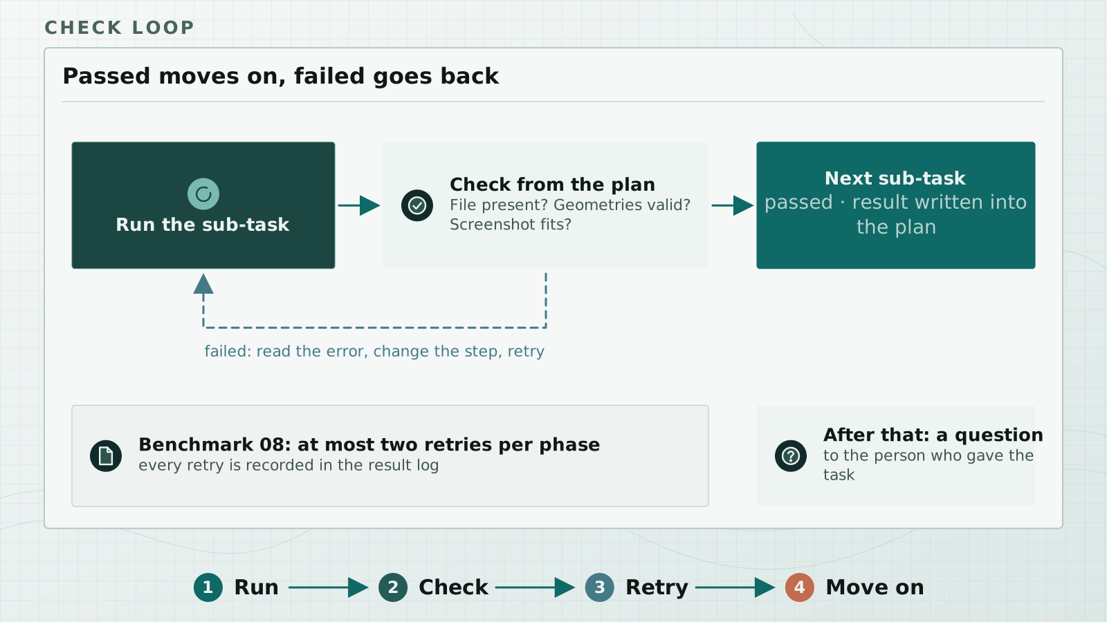
The plan names a check for every sub-task before the work begins. Is the file there? Are the geometries valid? Does the screenshot show the map the task asks for?
If the result passes, the coding agent writes it into the plan and moves to the next sub-task.
If it does not pass, the coding agent goes back. It reads the error message, changes the step and runs it again. Benchmark 8 allows at most two retries per phase for this, and every retry is recorded in the result log.
If the retry does not carry either, the loop ends at a question to the person. That is the rule from the first section: the loop ends at a checked result or at a question.
What such a plan looks like in a measurement series is shown by Benchmark 8.
Evidence
Concept 07 · part 4
The plan in Benchmark 08
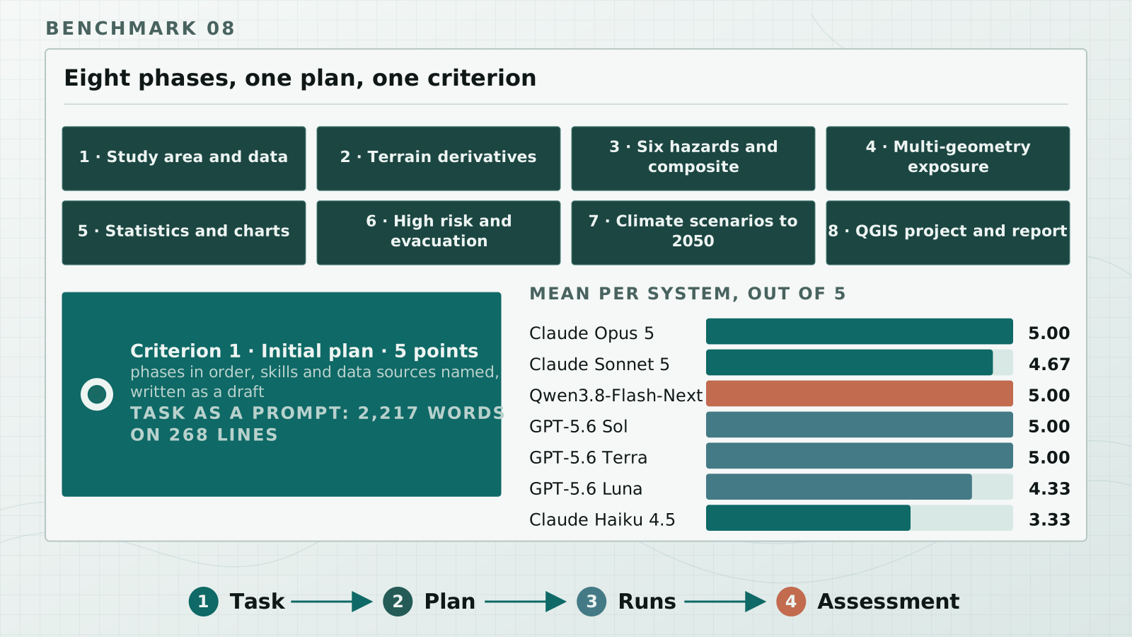
The task of Benchmark 8 comes in eight phases, which begin with the study area, the data and the terrain derivatives. Then come six hazards and their composite, multi-geometry exposure as well as statistics and charts. The end is high risk and evacuation, the climate scenarios to 2050 and the QGIS project with its report. Every phase ends with a screenshot.
The task demands a plan before the work, and the first criterion of the assessment gives five points for it. The plan names the phases in their order and the skills and data sources used, and it reads as a draft, not as a summary written afterwards.
Four of the seven systems took the full five points in all three runs; at the lower end stood Haiku with a mean of just over three points.
The plan is the cheap part of the work. Whether parts of it can run side by side is shown on the next slide.
Evidence
Concept 07 · part 5
Independent parts as further SpatialAgents
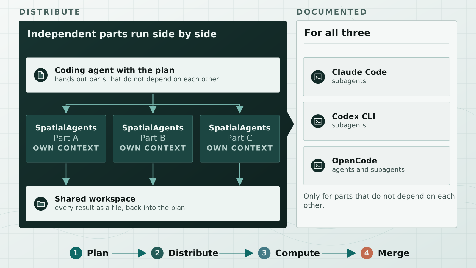
Some sub-tasks do not depend on each other. The six hazard indices in Benchmark 8 are an example: each comes from the base data, none from another index.
For such parts a coding agent can start further SpatialAgents. Each gets a task of its own and a context of its own. All of them work in the shared workspace and write their result as a file. The plan stays with the coding agent that started them. It merges the results and moves to the next sub-task.
The gain lies in the context. The tool results of one part land in the context of the further SpatialAgents, not in the main context.
All three coding agents document this as subagents.
What happens after the approval is shown by one task, start to finish.
Evidence
Concept 08 · System
One task, start to finish
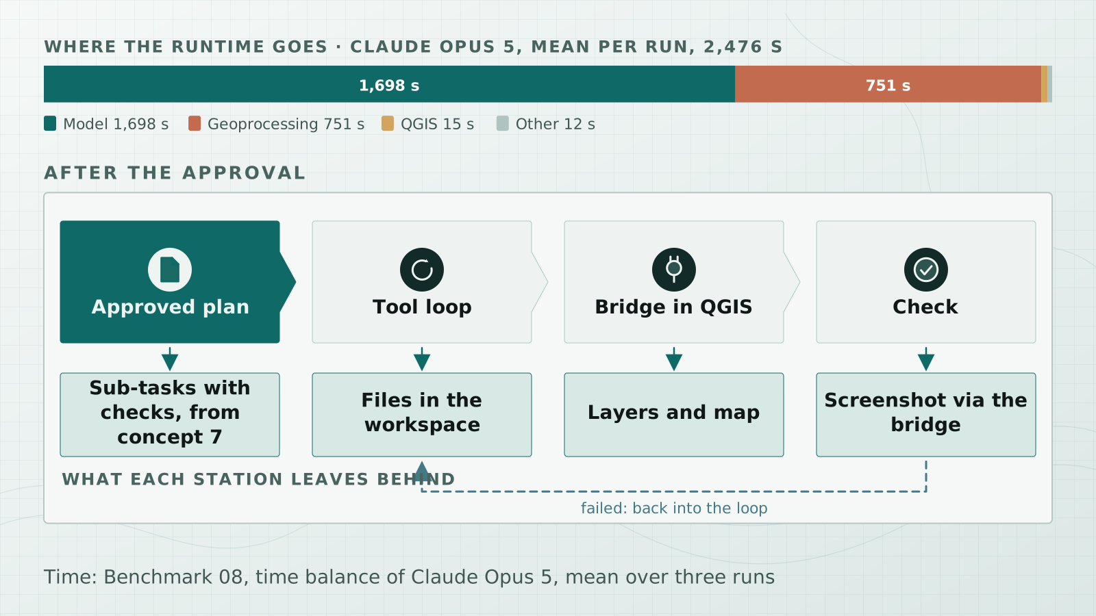
The plan is approved. What happens then has three stations and a check.
First the tool loop runs: the coding agent calls tools, and files appear in the workspace. The workspace is the shared directory for SpatialAgents and QGIS, and computing there is done with Python and on the command line.
Then the bridge acts in QGIS, where the files become layers and the layers become a map.
At the end comes the check the plan names for this sub-task. The bridge fetches a screenshot and the details of the layers from QGIS, and if the result does not fit, it goes back into the loop.
The time is spread unevenly. For Opus, of a good forty minutes of runtime, more than two thirds went to the model on average, just under a third to geoprocessing and only a few seconds to QGIS.
How short the computing part turns out depends on the library it is done with.
Evidence
Concept 09 · System
Geospatial API and token efficiency
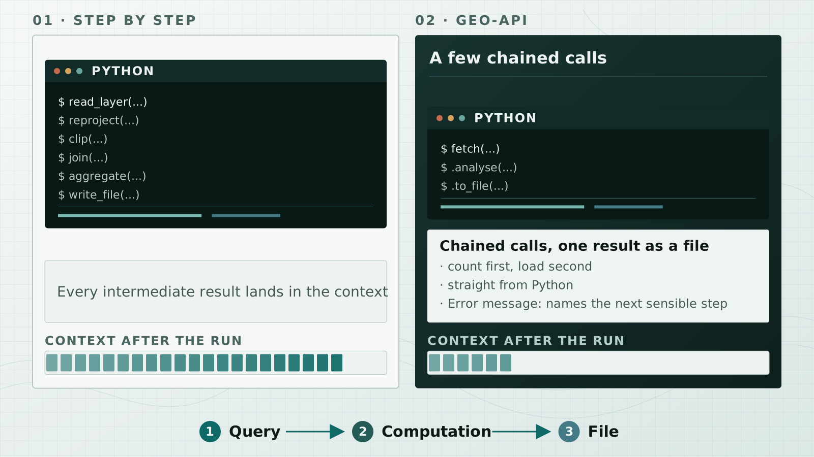
The Geospatial API, Geo-API for short, is a Python library, written to be used by agents. One call fetches data, a second computes, and a third writes the result as a file.
Without it, the same work becomes a long chain of single steps, in which every step delivers an intermediate result and every intermediate result lands in the context.
Four properties lower the token cost. The calls are declarative and can be chained. How many features a query matches can be counted before anything is loaded. Error messages name the next sensible step. And the call goes straight out of Python or from the command line, with no detour through a tool wrapper.
The Geo-API was available in the runs of the measurement series.
That describes the computing part. The way back into QGIS runs through the plugin and the bridge.
Evidence
Concept 10 · System
Plugin and bridge
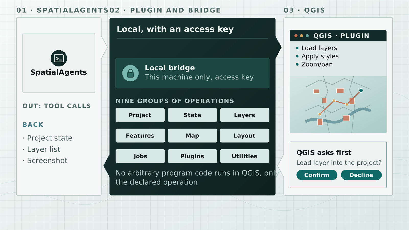
The plugin makes the open QGIS project reachable for SpatialAgents. It opens a connection that is valid only on this machine and demands an access key.
Tool calls arrive through this connection, and the bridge turns them into QGIS operations: it loads layers, styles them, moves the map and builds print layouts.
Three things go back, namely the state of the project, the list of layers and an image of the map. That image is how a coding agent looks at its own result.
Two limits apply here. QGIS puts any step that changes the project to the user for confirmation, and no arbitrary program code runs in QGIS, only the declared operation.
The computing therefore happens somewhere else.
Evidence
Concept 11 · System
Control and compute
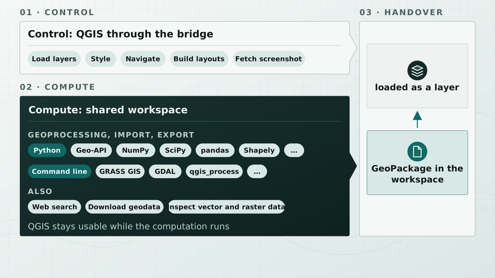
SpatialAgents separate two kinds of work: the control of QGIS and the computing with geodata.
Control runs through the bridge: loading layers, styling them, moving the map, building a print layout, fetching a screenshot.
Computing runs in the workspace: Python libraries, command-line tools, plus web search, downloading geodata and inspecting existing vector and raster data.
That has two consequences. QGIS stays usable, because no long computation holds up the interface. And every result lies there as a file that can be opened and recomputed independently of the project.
At one point the two lanes meet. A GeoPackage is created in the workspace, and the bridge loads it as a layer into the project.
One question is still open. Where the language model does its computing.
Evidence
Concept 12 · Operation and evidence
Local or cloud
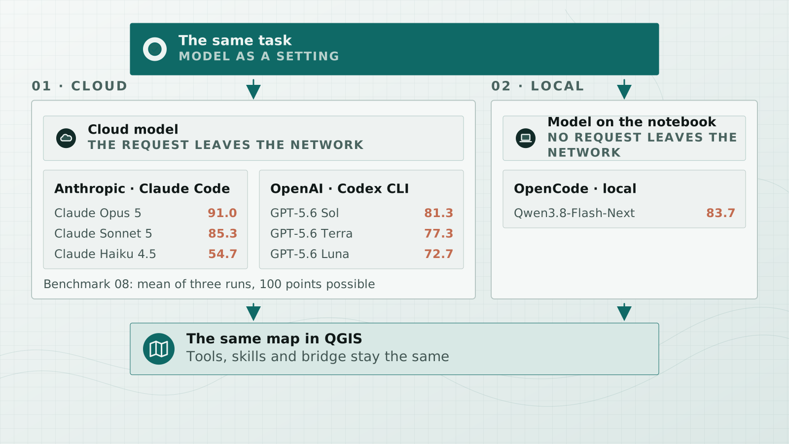
Which language model does the work is a setting. The same task runs with a model in the cloud or with a model on your own notebook, while tools, skills and the connection to QGIS stay the same.
The final section presents a series of measurements, Benchmark 8. It measured both routes and scored every run against the same criteria on a scale of a hundred points. Seven systems of agent and model solved the same hazard and climate analysis for Stuttgart, each of them three times.
One of these models sat on a desk: Qwen ran on a notebook, reached almost 84 of a hundred points and so finished ahead of all three cloud models from OpenAI.
In local operation no request leaves your own network, and both routes lead to the same QGIS map.
Whether a system solves the task is decided by the measurement.
Evidence
Concept 13 · Operation and evidence
Evidence through measurement series
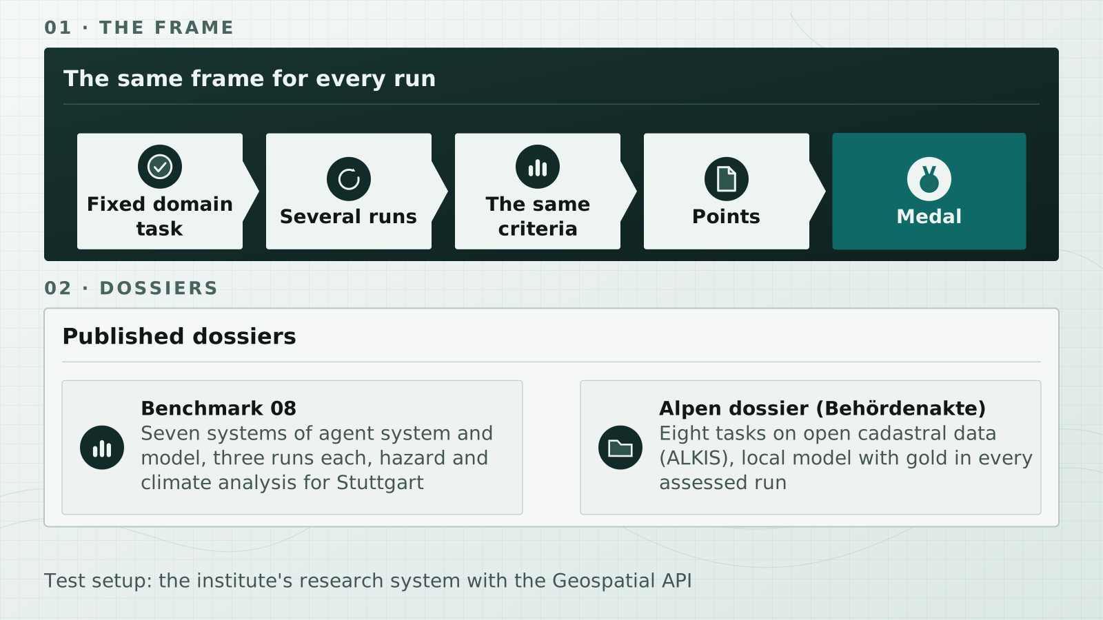
Whether a system solves a task is shown by a measurement series, and that is what benchmarks are for.
A benchmark is a fixed domain task with an assessment framework. Every model works on it several times, every run is assessed by the same criteria, and from the points comes a medal.
Two dossiers are published. The first is called Benchmark 8: seven systems of agent and model solve the same hazard and climate analysis for Stuttgart, each system three times.
The second is the Alpen dossier, the Behördenakte Alpen, with eight tasks from the daily work of an office on open cadastral data, ALKIS, of the municipality of Alpen on the Lower Rhine. Sonnet from the cloud met Qwen on a notebook, and the local model took gold in every assessed run.
The runs used the research system with additional domain skills for geoprocessing and the Geospatial API.
The two dossiers show the results in detail.
Evidence
- Benchmark 08: seven systems and their runs
- Benchmark 08: task and scoring criteria
- Alpen dossier: results of the eight tasks (German)
Concept 13 · part 2
Benchmark 08: points by model
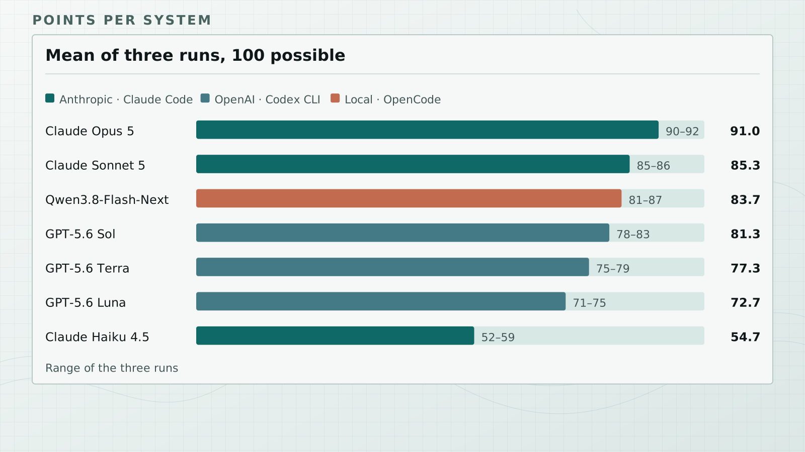
Benchmark 8 measured seven systems. Each system ran three times, and every run received points on a scale up to a hundred. The range of the three runs stands beside every bar.
The range is wide: in front is Opus with a mean of 91 points, at the end Haiku with just under 55, and in between stand Sonnet, Sol, Terra and Luna.
In third place stands the local model. Qwen reaches almost 84 points and so finishes ahead of all three cloud models from OpenAI, although it ran on a notebook.
What the runs cost in tokens and money is on the next slide.
Evidence
Concept 13 · part 3
Benchmark 08: tokens and cost per run
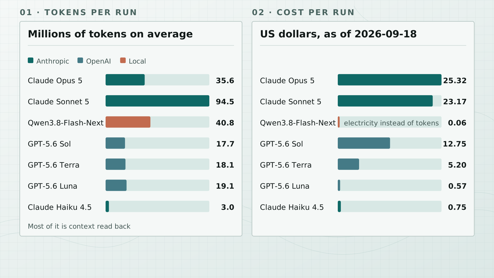
The same task consumes very different amounts of context depending on the model.
Sonnet reads the most with a good 94 million tokens per run, Haiku the least with three million; the three models from OpenAI sit at just under 20 million. Most of it is context read back, not output.
In money, as of September 2026: the dearest run costs a good 25 US dollars with Opus, the cheapest cloud run a little over half a dollar with Luna. The local run with Qwen pays for electricity instead of tokens, six cents.
More tokens do not mean more points, because Sonnet reads almost three times as much as Opus and scores less.
How many tool calls stand behind that, and how long a run takes, is on the next slide.
Evidence
Concept 13 · part 4
Benchmark 08: tool calls and runtime
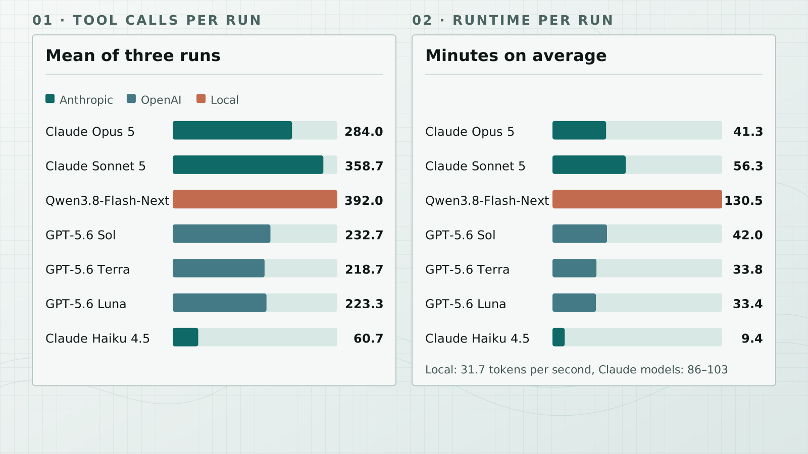
A run consists of hundreds of tool calls. Qwen needs the most with almost 400 per run, Haiku the fewest with a good 60, and the other five models lie between 220 and 360.
Runtime is measured by the wall clock. Haiku is done after a good nine minutes, Qwen takes the longest at almost 130 minutes, and the cloud models from OpenAI and Anthropic lie between half an hour and an hour.
For the local model most of the time goes to the model itself, because it runs at a good 30 tokens per second, while the Claude models reach 86 to 103.
More calls do not mean more time: Sol needs fewer calls than Opus and still finishes later.
The benchmark dossier shows the runs in detail.
Evidence
Next
Where to go from here.
This site shows the current state of research and development on the system. Projects, setup, training and support are provided by Geoinformatikbüro Dassau GmbH (GBD) ↗.